

One of my favorite Google tools is Sheets. I use it for much more than just data spreadsheets. There are many tweaks that make Sheets extra cool. Conditional formatting, charts, cell formatting, and more. One of the things that is easy to do but can be labor intensive is alternating row colors for a whole sheet. The good news is that there is a quick and easy way to do this with conditional formatting! Follow the steps below to alternate colors for rows or columns in an entire spreadsheet.
Change Row or Column Colors in Sheets
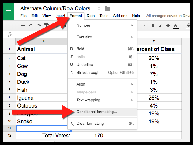
- In Google Sheets, click on “Format” and then click on “Conditional Formatting”.
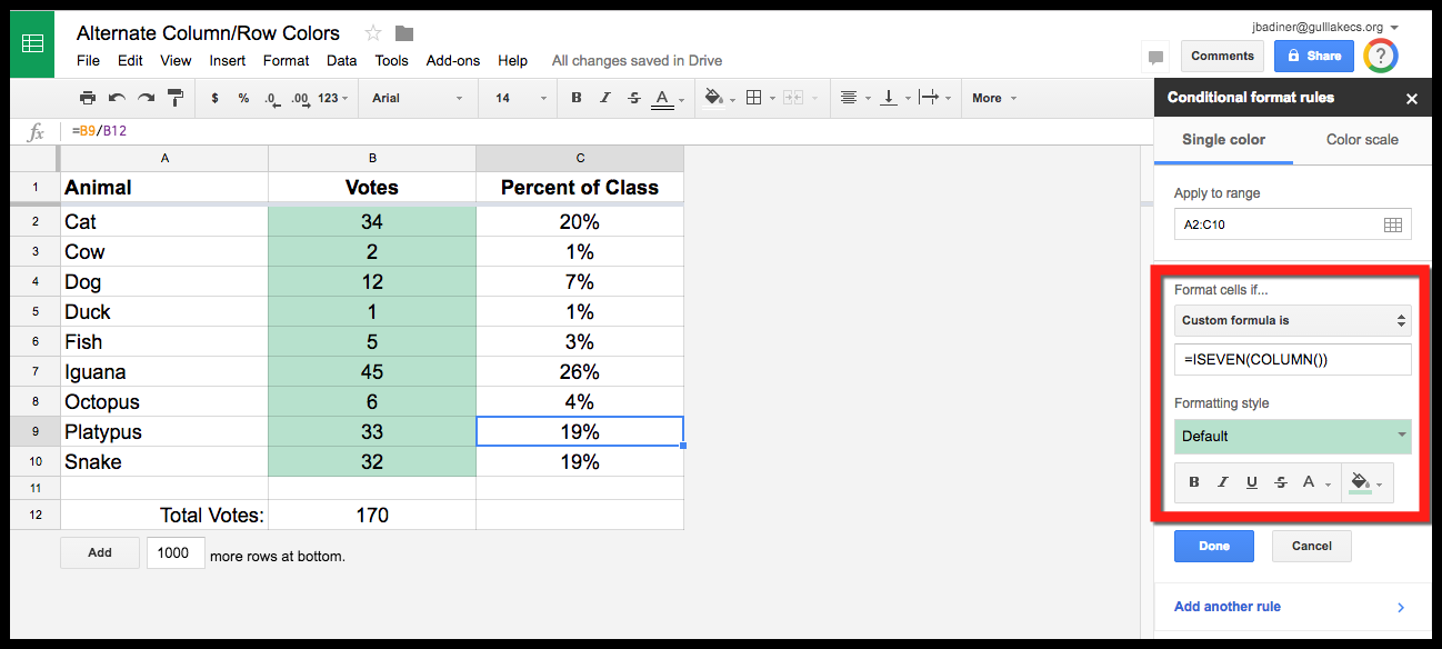
- Select the range using the “Apply to range” field.

- Under the “Format cells if…” dropdown menu select “Custom formula is”.
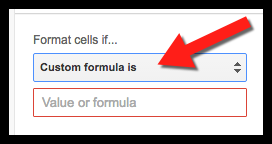
- Here is where you select which rows or columns you want to have what type of formatting (see “Apply Formatting to Rows” or “Apply Formatting to Columns” section below).
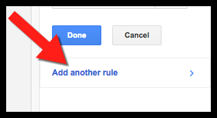
- After setting one row or column color click “Add another rule” at the bottom.
Apply Formatting to Rows:
- To apply a color to all even rows, type =ISEVEN(ROW()).

- To apply the rule to odd rows, type =ISODD(ROW()).

- Set your formatting style in the “Formatting style” box.
Apply Formatting to Columns:
- To apply color to all even columns, type =ISEVEN(COLUMN()).
- To apply the rule to odd columns, type =ISODD(COLUMN()).

- Set your formatting style in the “Formatting style” box.
Open up a Google Sheets and give it a try!
Get these steps as a document Here!